
今回は、Pythonの算術演算のうちmathモジュールを使った三角関数関連についてまとめます。
- 円周率πの定義、角度変換(ラジアン⇔度)
- 三角関数、逆三角関数
- 極座標系との変換
使用例として、それぞれmatplotlibモジュールを使ったグラフも併せて載せています。
環境
- OS: Ubuntu16.04LTS
- Python3.7.2@Anaconda
定数:π
πは下記の通り定数として定義されています。
>>> import math
>>> math.pi
3.141592653589793
※他にも定数や固定値として定義されているものがありますので、別途まとめる予定です。
角度変換 ラジアン⇔度
三角関数の計算は基本的にラジアンを使いますので、角度が(度)の場合は(ラジアン)に変換が必要です。ここでは、変換するための関数を示します。
角度(度) → (ラジアン)変換
math.radians(x)を使います。返り値は浮動小数点です。
# 60°をラジアンに変換
>>> math.radians(60)
1.0471975511965976

# 180°をラジアンに変換
>>> math.radians(180)
3.141592653589793

# 180° = πですね
>>> math.radians(180) == math.pi
True
角度(ラジアン) → (度)変換
math.degrees(x)を使います。こちらも返り値は浮動小数点です。
>>> math.degrees(math.pi)
180.0
>>> math.degrees(math.pi / 4)
45.0
三角関数いろいろ
正弦 \(y=sin(x)\)
math.sin(x)を使います。引数xの単位は、[rad](ラジアン)です。
>>> import math
>>> x = 1.23
>>> math.sin(x)
0.9424888019316975

# 度の場合はラジアンに変換します
>>> d = 60
>>> math.sin(math.radians(d))
0.8660254037844386
余弦 \(y=cos(x)\)
math.cos(x)を使います。引数xの単位は、[rad](ラジアン)です。
>>> import math
>>> x = 1.23
>>> math.cos(x)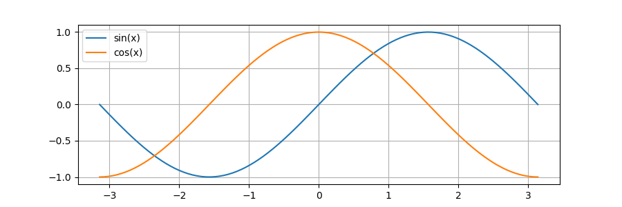
0.3342377271245026これだけだと面白くないのでmatplotlibでグラフを書いてみます。
import matplotlib.pyplot as plt
import numpy as np
import math

# グラフの大きさの設定
plt.figure(figsize=(9, 3))

# x軸の値を生成(-π≦x≦π)
x = np.linspace(-math.pi, math.pi, 100)

# sin(x) ※np.sin(x)を使うともっと簡単に書けますがここではmathモジュールを使います。
y1 = [math.sin(val) for val in x]

# cos(x) ※np.cos(x)を使うともっと簡単に書けますがここではmathモジュールを使います。
y2 = [math.cos(val) for val in x]

# 凡例の設定
plt.plot(x, y1, label = "sin(x)")
plt.plot(x, y2, label = "cos(x)")

# 補助線の設定
plt.grid(True)

# グラフの描画
plt.show()
\(sin(x)\)と\(cos(x)\)のグラフを重ねてみました。
※matplotlibについては別途まとめる予定です。
正接 \(y=tan(x)\)
math.tan(x)を使います。引数xの単位は、[rad](ラジアン)です。
>>> import math
>>> x = 1.23
>>> math.tan(1.23)
2.819815734268152
こちらもグラフを書いてみます。
import matplotlib.pyplot as plt
import numpy as np
import math

# グラフの大きさの設定
plt.figure(figsize=(9, 3))

# x軸の値を生成(-π/2<x<π/2)
x = np.linspace(-math.pi/2, math.pi/2, 100, endpoint=False)

# tan(x) ※np.tan(x)を使うともっと簡単に書けますがここではmathモジュールを使います。
y = [math.tan(val) for val in x]

plt.plot(x, y, label = "tan(x)")
plt.ylim(-10, 10)
plt.grid(True)

plt.legend()
plt.show()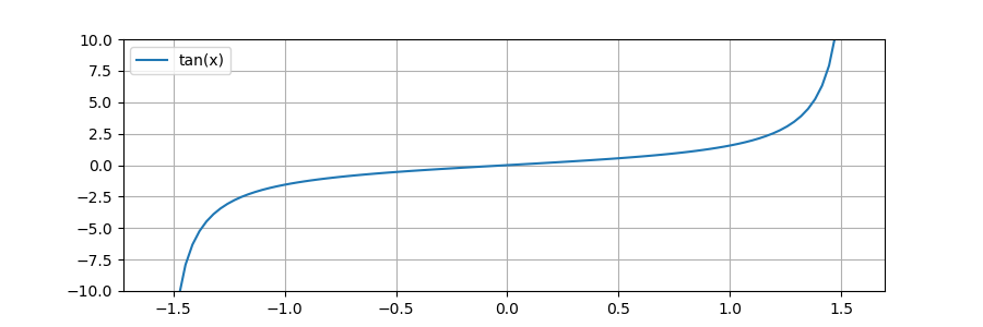
三角関数の応用
逆正弦 \(y=arcsin(x)\)
math.asin(x)を使います。
x の逆正弦\(arcsin(x)\)を返します。単位は(ラジアン)です。
>>> import math
# まずはsin(0.5)を計算
>>> y = math.sin(0.5)
>>> y
0.479425538604203

# arcsinで元のxに等しいことが確認できます。
>>> math.asin(y)
0.5
逆余弦 \(y=arccos(c)\)
math.acos(x)を使います。
x の逆余弦\(arccos(c)\)を返します。単位は(ラジアン)です。
>>> import math
# まずはcos(0.5)を計算
>>> y = math.cos(0.5)
>>> y
0.8775825618903728
# arccosで元のxに等しいことが確認できます。
>>> math.acos(y)
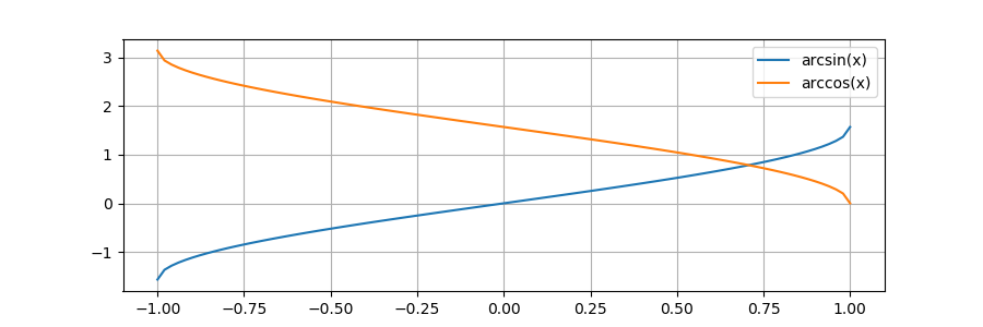
0.4999999999999999グラフは以下です。(with matplotlib)
逆正接 \(y=arctan(x)\)
math.atan(x)を使います。
x の逆正接\(arctan(x)\)を返します。単位は(ラジアン)です。
>>> y = math.tan(1)
>>> y
1.5574077246549023
>>> math.atan(y)
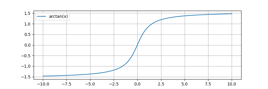
1.0グラフは以下です。(with matplotlib)
その他三角関数
直交座標系\((x,y)\)から極座標系\((r, θ)\)へ変換する関数もあります。
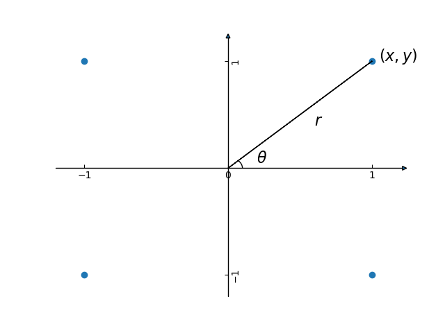
ベクトル\((x, y)\)の長さ:\(r\)
ベクトル\((x, y)\)の長さ(ユークリッドノルム:\( r=\sqrt{x^2+y^2} \))は、math.hypot(x, y)を使うと簡単に求まります。
>>> math.hypot(3, 4)
5.0
>>> math.hypot(1, 1)
1.4142135623730951
ベクトル\((x, y)\)が\(x\)軸となす角度:\(θ\)
ベクトル\((x, y)\)が\(x\)軸となす角度(\(θ=arctan(y/x)\))はmath.atan2(y, x)を使います。戻り値は -\(π\)から\(π\)の間になります。
引数は符号(+/-)を記載できるため角度の象限も計算できます。xとyの順番に注意!
# 第一象限
>>> theta = math.atan2(1,1)
>>> theta
0.7853981633974483  # math.degrees(theta) >>> 45.0

# 第二象限
>>> theta = math.atan2(1,-1)
>>> theta
2.356194490192345 # math.degrees(theta) >>> 135.0

# 第三象限
>>> theta = math.atan2(-1,1) #
>>> theta
-0.7853981633974483 # math.degrees(theta) >>> -45.0

# 第四象限
>>> theta = math.atan2(-1,-1)
>>> theta
-2.356194490192345 # math.degrees(theta) >>> -135.0
まとめ
今回は、Pythonの数値演算のうち三角関数の使い方について、mathモジュールを使った角度変換(ラジアン⇔度)、三角関数、逆三角関数そして極座標系との変換方法について、それぞれのグラフ描画も示しながらまとめました。